Biopython
What is Biopython?
Biopython is the largest and most common bioinformatics package for Python. It contains a number of different sub-modules for common bioinformatics tasks.
It is freely available here:
while the entire source code is hosted here:
Note
The Biopython code is distributed under the Biopython License.
Biopython sports several features. It provides:
Data structures for biological sequences and features thereof, as well as a multitude of manipulation functions for performing common tasks, such as translation, transcription, weight computations, ...
Functions for loading biological data into
dict-like data structures.Supported formats include, for instance: FASTA, PDB, GenBank, Blast, SCOP, PubMed/Medline, ExPASy-related formats
Functions for data analysis, including basic data mining and machine learning algorithm: k-Nearest Neighbors, Naive Bayes, and Support Vector Machines
Access to online services and database, including NCBI services (Blast, Entrez, PubMed) and ExPASY services (SwissProt, Prosite)
Access to local services, including Blast, Clustalw, EMBOSS.
Warning
In order to use local services (such as Blast), the latter must be properly installed and configured on the local machine.
Setting up the local services is beyond the scope of this course.
Note
In order to install Biopython:
On a Debian-based distributions (for instance Ubuntu), just type:
$ sudo apt-get install python-biopython
On a generic GNU/Linux distribution, just type:
$ pip install biopython --user
Please refer to the official documentation for further instructions.
Note
While Biopython is the main player in the field, it is not the only one. Other interesting packages are:
ETE and DendroPy, dedicated to computation and visualization of phylogenetic trees.
CSB for dealing with sequences and structures, computing alignments and profiles (with profile HMMs), and Monte Carlo sampling.
biskit is designed for structural bioinformatics tasks, such as loading 3D protein structures in Protein Data Bank (PDB) format, homology modelling, molecular dynamics simulations (using external simulators) and trajectory computations, and docking, among others.
You are free to mix and match all the packages you need.
Biopython: Sequences
Sequences lay at the core of bioinformatics: although DNA, RNA and proteins are molecules with specific structures and dynamical behaviors, their basic building block is their sequence.
Biopython encodes sequences using objects of type Seq, provided by the
Bio.Seq sub-module. Take a look at their manual:
from Bio.Seq import Seq
help(Seq)
Note
The official documentation of the Biopython Seq class can be found on
the Biopython wiki.
Each Seq object is associated to a formal alphabet.
- Each sequence has its own alphabet
- Conversions between different sequence types (transcription, translation) can be seen as a change of alphabet.
- Some operations (e.g. concatenation) can not be done between sequences with incompatible alphabets.
The various alphabets supported by Biopython can be found in Bio.Alphabet,
e.g. Bio.Alphabet.IUPAC.
The most basic alphabets are:
IUPAC.unambiguous_dna: a sequence of DNAIUPAC.unambiguous_rna: a sequence of RNAIUPAC.protein: a protein sequence
Example. To create a generic sequence, i.e. a sequence not bound to any specific alphabet, write:
>>> from Bio.Seq import Seq
>>> s = Seq("ACCGTTTAAC") # no alphabet specified
>>> print type(s)
<class 'Bio.Seq.Seq'>
>>> s
Seq('ACCGTTTAAC', Alphabet())
>>> print s
ACCGTTTAAC
To create a DNA sequence, specify the corresponding alphabet when creating
the Seq object:
>>> from Bio.Seq import Seq
>>> from Bio.Alphabet import IUPAC
>>> s = Seq("ACCGTTTAAC", IUPAC.unambiguous_dna)
>>> s
Seq('ACCGTTTAAC', IUPACUnambiguousDNA())
Seq objects act mostly like standard Python strings str. For instance,
you can write:
>>> from Bio.Seq import Seq
>>> s = Seq("ACTG")
>>> len(s)
4
>>> s[2]
'T'
>>> s[1:-1]
Seq('CT', Alphabet())
>>> s.count("C")
3
However, some operations are restricted to Seq objects with the same
alphabet (in order to prevent the user from, say, concatenating nucleotides
and amino acids):
>>> s = Seq("ACTG", IUPAC.unambiguous_dna)
>>> s + s
Seq('ACTGACTG', IUPACUnambiguousDNA())

>>> t = Seq("AAADGHHHTEWW", IUPAC.protein)
>>> s
Seq('ACTG', IUPACUnambiguousDNA())
>>> t
Seq('AAADGHHHTEWW', IUPACProtein())
>>> s + t
Traceback (most recent call last):
  File "<stdin>", line 1, in <module>
  File "/home/stefano/.local/lib/python2.7/site-packages/Bio/Seq.py", line 292, in __add__
    self.alphabet, other.alphabet))
TypeError: Incompatible alphabets IUPACUnambiguousDNA() and IUPACProtein()
To convert back a Seq object into a normal str object, just use the
normal type-casting operator str():
>>> s = Seq("ACTG", IUPAC.unambiguous_dna)
>>> str(s)
Warning
Just like strings, Seq objects are immutable:
>>> s = Seq("ACCGTTTAAC")
>>> s[0] = "G"
Traceback (most recent call last):
  File "<stdin>", line 1, in <module>
TypeError: 'Seq' object does not support item assignment
Thanks to their immutability, Seq objects can be used as keys in
dictionaries (like str objects do).
Note
Biopython also provides a mutable sequence type MutableSeq.
You can convert back and forth between Seq and MutableSeq:
>>> s = Seq("ACTG", IUPAC.unambiguous_dna)
>>> muts = s.tomutable()
>>> muts[0] = "C"
>>> muts
MutableSeq('CCTG', IUPACUnambiguousDNA())
>>> muts.toseq()
Seq('CCTG', IUPACUnambiguousDNA())
Some operations are only available when specific alphabets are used. Let’s see a few examples.
Example. The complement() method allows to complement a DNA or RNA
sequence:
>>> s = Seq("CCGTTAAAAC", IUPAC.unambiguous_dna)
>>> s.complement()
Seq('GGCAATTTTG', IUPACUnambiguousDNA())
while the reverse_complement() also reverses the result from left
to right:
>>> s.reverse_complement()
Seq('GTTTTAACGG', IUPACUnambiguousDNA())
Warning
Neither of these methods is available for other alphabets:
>>> p = Seq("ACLKQ", IUPAC.protein)
>>> p.complement()
Traceback (most recent call last):
  File "<stdin>", line 1, in <module>
  File "/home/stefano/.local/lib/python2.7/site-packages/Bio/Seq.py", line 760, in complement
    raise ValueError("Proteins do not have complements!")
ValueError: Proteins do not have complements!
Example. (Adapted from the Biopython tutorial.) Transcription is the biological process by which a DNA sequence is transcribed into the corresponding DNA.
A picture of the transcription process:
5’  ATGGCCATTGTAATGGGCCGCTGAAAGGGTGCCCGATAG 3’ (coding strand)
    |||||||||||||||||||||||||||||||||||||||
3’  TACCGGTAACATTACCCGGCGACTTTCCCACGGGCTATC 5’ (template strand)
                        |
                   Transcription
                        ↓
5’  AUGGCCAUUGUAAUGGGCCGCUGAAAGGGUGCCCGAUAG 3’ (mRNA)
The same process can be “simulated” on Seq objects. Starting from the
coding strand (as is usually done in bioinformatics), it is only a matter
of converting T’s into U’s:
>>> coding_dna
Seq('ATGGCCATTGTAATGGGCCGCTGAAAGGGTGCCCGATAG', IUPACUnambiguousDNA())
>>> mrna = coding_dna.transcribe()
>>> mrna
Seq('AUGGCCAUUGUAAUGGGCCGCUGAAAGGGUGCCCGAUAG', IUPACUnambiguousRNA())
From the template strand instead we first have to compute the reverse complement, and then perform the character substitution:
>>> template_dna
'TACCGGTAACATTACCCGGCGACTTTCCCACGGGCTATC'
>>> template_dna.reverse_complement().transcribe()
Seq('AUGGCCAUUGUAAUGGGCCGCUGAAAGGGUGCCCGAUAG', IUPACUnambiguousRNA())
It is also easy to perform the reverse process, back-transcription:
>>> mrna
'AUGGCCAUUGUAAUGGGCCGCUGAAAGGGUGCCCGAUAG'
>>> mrna.back_transcribe()
Seq('ATGGCCATTGTAATGGGCCGCTGAAAGGGTGCCCGATAG', IUPACUnambiguousDNA())
Warning
These functions also take care of checking that the input alphabet is the right one (e.g. DNA) and apply the right alphabet to the result (e.g. RNA).
Example. (Adapted from the Biopython tutorial.) Let’s not take a look at translation, i.e. mRNA to protein.
The code is as follows:
>>>from Bio.Seq import Seq
>>>from Bio.Alphabet import IUPAC
>>>mrna = Seq("AUGGCCAUUGUAAUGGGCCGCUGAAAGGGUGCCCGAUAG", IUPAC.unambiguous_rna)
>>>print mrna
AUGGCCAUUGUAAUGGGCCGCUGAAAGGGUGCCCGAUAG
>>>print mrna.translate()
MAIVMGR*KGAR*
Here the stop codons are indicated with an asterisk "*".
Now, different coding tables are available, for instance:
>>> coding_dna.translate(table="Vertebrate Mitochondrial")
Seq('MAIVMGRWKGAR*', HasStopCodon(IUPACProtein(), '*'))
It’s also possible to tell the translate() method to stop at the first
stop codon:
>>> coding_dna.translate()
Seq('MAIVMGR*KGAR*', HasStopCodon(IUPACProtein(), '*'))
>>> coding_dna.translate(to_stop=True)
Seq('MAIVMGR', IUPACProtein())
In this case the stop codon is not included in the resulting sequence.
Note
The Genetic Codes page of the NCBI provides the full list of translation tables used by Biopython.
In order to visualize the various translation tables, you can do:
from Bio.Data import CodonTable

ttable = CodonTable.unambiguous_dna_by_name["Standard"]
print ttable

ttable = CodonTable.unambiguous_dna_by_name["Vertebrate Mitochondrial"]
print ttable
You can also visualize what are the encodings of stop and start codons:
print ttable.stop_codons
print ttable.start_codons
Let’s take a look at some common sequence formats.
FASTA is the most basic format, we have used it several times already:
>sp|P25730|FMS1_ECOLI CS1 fimbrial subunit A precursor (CS1 pilin)
MKLKKTIGAMALATLFATMGASAVEKTISVTASVDPTVDLLQSDGSALPNSVALTYSPAV
NNFEAHTINTVVHTNDSDKGVVVKLSADPVLSNVLNPTLQIPVSVNFAGKPLSTTGITID
SNDLNFASSGVNKVSSTQKLSIHADATRVTGGALTAGQYQGLVSIILTKST
>sp|P15488|FMS3_ECOLI CS3 fimbrial subunit A precursor (CS3 pilin)
MLKIKYLLIGLSLSAMSSYSLAAAGPTLTKELALNVLSPAALDATWAPQDNLTLSNTGVS
NTLVGVLTLSNTSIDTVSIASTNVSDTSKNGTVTFAHETNNSASFATTISTDNANITLDK
NAGNTIVKTTNGSQLPTNLPLKFITTEGNEHLVSGNYRANITITSTIK
GenBank is a richer sequence format for genes, it includes fields for various kinds of annotations (e.g. source organism, bibliographical references, database-specific accession number).
A GenBank file looks like this:
LOCUS       5I3U_F                    39 bp    DNA     linear   SYN 31-AUG-2016
DEFINITION  Chain F, Structure Of Hiv-1 Reverse Transcriptase N-site Complex;
            Catalytic Incorporation Of Aztmp To A Dna Aptamer In Crystal.
ACCESSION   5I3U_F
VERSION     5I3U_F
KEYWORDS    .
SOURCE      synthetic construct
  ORGANISM  synthetic construct
            other sequences; artificial sequences.
REFERENCE   1  (bases 1 to 39)
  AUTHORS   Tu,X., Das,K., Han,Q., Bauman,J.D., Clark AD,Jr., Hou,X.,
            Frenkel,Y.V., Gaffney,B.L., Jones,R.A., Boyer,P.L., Hughes,S.H.,
            Sarafianos,S.G. and Arnold,E.
  TITLE     Structural basis of HIV-1 resistance to AZT by excision
  JOURNAL   Nat. Struct. Mol. Biol. 17 (10), 1202-1209 (2010)
   PUBMED   20852643
...
FEATURES             Location/Qualifiers
     source          1..39
                     /organism="synthetic construct"
                     /mol_type="other DNA"
                     /db_xref="taxon:32630"
ORIGIN
        1 taatacncnc ccttcggtgc tttgcaccga agggggggn
//
UniProt (obtained by combining SwissProt, TrEMBL and PIR) is the GenBank equivalent for protein sequences:
ID  143B_HUMAN  STANDARD; PRT; 245 AA.
AC  P31946;
DT  01-JUL-1993 (Rel. 26, Created)
DT  01-FEB-1996 (Rel. 33, Last sequence update)
DT  15-SEP-2003 (Rel. 42, Last annotation update)
DE  14-3-3 protein beta/alpha (Protein kinase C inhibitor protein-1)
DE  (KCIP-1) (Protein 1054).
GN  YWHAB.
OS  Homo sapiens (Human).
OC  Eukaryota; Metazoa; Chordata; Craniata; Vertebrata; Euteleostomi;
OC  Mammalia; Eutheria; Primates; Catarrhini; Hominidae; Homo.
OX  NCBI_TaxID=9606;
RN  [1]
RP  SEQUENCE FROM N.A.
RC  TISSUE=Keratinocytes;
RX  MEDLINE=93294871; PubMed=8515476;
RA  Leffers H., Madsen P., Rasmussen H.H., Honore B., Andersen A.H.,
RA  Walbum E., Vandekerckhove J., Celis J.E.;
RT  "Molecular cloning and expression of the transformation sensitive
RT  epithelial marker stratifin. A member of a protein family that has
RT  been involved in the protein kinase C signalling pathway.";
The Bio.SeqIO module provides a functions to parse all of the above
(among others).
In particular, the parse() function takes a file handle and the format
of the file (as a string) and returns an iterable of SeqRecord objects:
from Bio.SeqIO import parse
help(parse)

f = open("test.fasta")
for record in parse(f, "fasta"):
    print record.id, record.seq
Warning
An iterable is a function that allows to iterate over a collection of objects (similar to a list).
When given an iterator, you can either use it as in the code above:
iterable = get_it_from_somewhere() # e.g. parse()
for element in iterable:
    do_something(element)
or extract one element at a time, with the next() method:
iterable = get_it_from_somewhere() # e.g. parse()
first_element = iterable.next()
do_something(first_element)
second_element = iterable.next()
do_something(second_element)
# ...
The iterable allows to iterate over a list of SeqRecord objects. The
SeqRecord objects associate a Seq sequence with additional meta-data,
such as human-readable descriptions, annotations, and sequence features:
>>> from Bio.SeqRecord import SeqRecord
>>> help(SeqRecord)
Each SeqRecord object provides these attributes:
.seq: the sequence itself, typically aSeqobject..id: the primary identifier of the sequence – a string..name: a “common” identifier for the sequence, also a string..description: a human readable description of the sequence..annotations: adictof additional information.
among others.
In order to read a SeqRecord object from a file:
>>> from Bio import SeqIO
>>> record = SeqIO.parse(open("sequences.fasta"), "fasta").next()
>>> record
SeqRecord(seq=Seq('METNCRKLVSACVQLGVQPAAVECLFSKDSEIKKVEFTDSPESRKEAASSKFFP...RPV', SingleLetterAlphabet()), ...
>>> record.id
'Q99697'
>>> record.name
'Q99697'
>>> record.annotations
{}
Here record.annotations is empty because the FASTA format does not really
support sequence annotations.
The very nice thing about the SeqIO and SeqRecord mechanism is that
they allow to process all of the different formats described above (FASTA,
GenBank, UniProt) using the very same code!
Let’s see what happens with a GenBank file:
>>> record = SeqIO.parse(open("data.genbank"), "genbank").next()
>>> record
SeqRecord(seq=Seq('TAATACNCNCCCTTCGGTGCTTTGCACCGAAGGGGGGGN', IUPACAmbiguousDNA()), ...
>>> from pprint import pprint
>>> pprint(record.annotations)
{'accessions': ['5I3U_F'],
 'data_file_division': 'SYN',
 'date': '31-AUG-2016',
 'keywords': [''],
 'organism': 'synthetic construct',
 'references': [Reference(title='Structural basis of HIV-1 resistance to AZT by excision', ...)],
 'source': 'synthetic construct',
 'taxonomy': ['other sequences', 'artificial sequences'],
 'topology': 'linear'}
This way, you can (almost) forget about the format of the sequence data you are working with – all the parsing is done automatically by Biopython.
Finally, the SeqIO.write() method allows to write a SeqRecord objects
or a list of SeqRecord objects to disk, in a given format:
fr = open("data.genbank", "r")
record = SeqIO.parse(fr, "genbank").next()

fw = open("seq1.fasta", "w)
SeqIO.write(record, fw, "fasta")
Biopython: Structures
Biopython allows to manipulate polypeptide structures via the Bio.PDB module.
We will focus on data coming from the Protein Data Bank (PDB):
The PDB is by far the largest protein structure resource available online. At the time of writing, it hosts more thank 120k distinct protein structures, including protein-protein, protein-DNA, protein-RNA complexes.
In order to load the required code, just type:
from Bio.PDB import *
Note
For the documentation of the Bio.PDB module, see:
Note
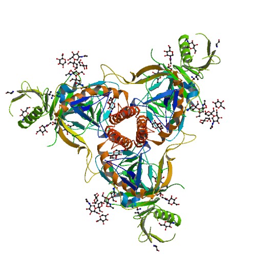
In the following we will use the Zaire Ebolavirus glicoprotein structure
5JQ3, available here:
This is what this structure looks like:
Protein Structure File Formats
The PDB distributes protein structures in two different formats:
The XML-based file format. It is not supported by Biopython.
The
mmciffile format. (The actual file extension is.cif.) See for instance:This is the most recent and “parsable” file format.
The
pdbfile format, which is a specially formatted text file. See for instance:This is the historical file format. It is (mostly) still distributed because of legacy tools that do not (yet) understand the newer and cleaner
mmciffiles.
Warning
Some (many?) PDB files distributed by the Protein Data Bank contain formatting errors that make them ambiguous or difficult to parse.
The Bio.PDB module attempts to deal with these errors automatically.
Of course, Biopython is not perfect, and some formatting errors may still make it do the wrong thing, or raise an exception.
Depending on your goal, you can either:
- manually correct the structure, e.g. if you have to analyze a single structure
- ignore the error, e.g. when you are just computing global statistics about a large number of structures, and a few errors do not really impact the overall numbers
We will see how to ignore these “spurious” errors soon.
The Bio.PDB module implements two different parsers, one for the pdb
format and one for the mmcif format. Let’s try them out.
Starting with:
>>> from Bio.PDB import *
To load a cif file, use the Bio.MMCIF.MMCIFParser module:
>>> parser = MMCIFParser()
>>> struct = parser.get_structure("5jq3", "5jq3.cif")
# four warnings
>>> struct
<Structure id=5jq3>
>>> print type(struct)
<class 'Bio.PDB.Structure.Structure'>
To load a pdb file, use the Bio.PDB.PDBParser module:
>>> parser = PDBParser()
>>> struct = parser.get_structure("5jq3", "5jq3.pdb")
# four warnings
>>> struct
<Structure id=5jq3>
>>> print type(struct)
<class 'Bio.PDB.Structure.Structure'>
As you can see, both parsers give you the same kind of object, a Structure.
The header of the structure is a dict which stores meta-data about the
protein structure, including its resolution (in Angstroms), name, author,
release date, etc.
To access it, write:
>>> print struct.header.keys()
['structure_method', 'head', 'journal', 'journal_reference',
'compound', 'keywords', 'name', 'author', 'deposition_date',
'release_date', 'source', 'resolution', 'structure_reference']
>>> print struct.header["name"]
crystal structure of ebola glycoprotein
>>> print struct.header["release_date"]
2016-06-29
>>> print struct.header["resolution"]
2.23   # Å
Warning
The header dictionary may be an empty, depending on the structure and
the parser. Try it out with the mmcif parser!
Note
You can download the required files directly from the PBD server with:
>>> pdbl = PDBList()
>>> pdbl.retrieve_pdb_file('1FAT')
Downloading PDB structure '1FAT'...
'/home/stefano/scratch/fa/pdb1fat.ent'
The file will be put into the current working directory.
The PDBList object also allows you to retrieve a full copy of the PDB
database, if you wish to do so. Note that the database takes quite a bit of
disk space.
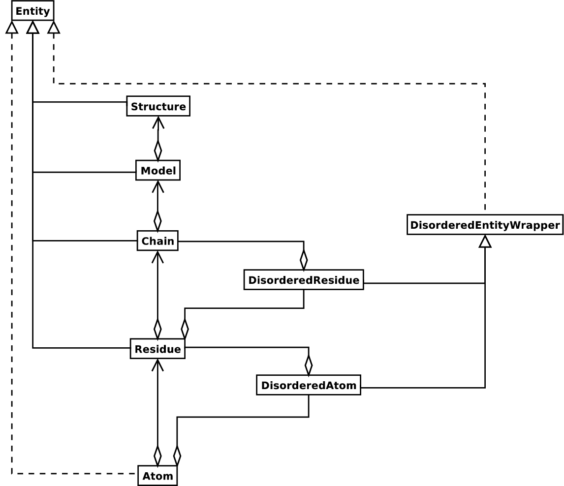
Structures as Hierarchies
Structural information is natively hierarchical.
The hierarchy is represented by Bio.PDB as follows (image taken from the
Biopython Structural Bioinformatics FAQ):
Example. For instance, the 5JQ3 PDB structure is composed of:
- A single model, containing
- Two chains:
- chain A, containing 338 residues
- chain B, containing 186 residues
- Each residue is composed by multiple atoms, each having a 3D position represented as by (x, y, z) coordinates.
- Two chains:
More specifically, here are the related Bio.PDB classes:
A
Structuredescribes one or more models, i.e. different 3D conformations of the very same structure (for NMR).The
Structure.get_models()method returns an iterator over the models:>>> it = struct.get_models() >>> it <generator object get_models at 0x7f318f0b3fa0> >>> models = list(it) >>> models [<Model id=0>] >>> type(models[0]) <class 'Bio.PDB.Model.Model'>
Here I turned the iterator into a proper list with the
list()function.A
Structurealso acts as adict: given a model ID, it returns the correspondingModelobject:>>> struct[0] <Model id=0>
A
Modeldescribes exactly one 3D conformation. It contains one or more chains.The
Model.get_chain()method returns an iterator over the chains:>>> chains = list(models[0].get_chains()) >>> chains [<Chain id=A>, <Chain id=B>] >>> type(chains[0]) <class 'Bio.PDB.Chain.Chain'> >>> type(chains[1]) <class 'Bio.PDB.Chain.Chain'>
A
Modelalso acts as adictmapping from chain IDs toChainobjects:>>> model = models[0] >>> model <Model id=0> >>> model["B"] <Chain id=B>
A
Chaindescribes a proper polypeptide structure, i.e. a consecutive sequence of bound residues.The
Chain.get_residues()method returns an iterator over the residues:>>> residues = list(chains[0].get_residues()) >>> len(residues) 338 >>> type(residues[0]) <class 'Bio.PDB.Residue.Residue'>
A
Residueholds the atoms that belong to an amino acid.The
Residue.get_atom()(unfortunately, “atom” is singular) returns an iterator over the atoms:>>> atoms = list(residues[0].get_atom()) >>> atoms [<Atom N>, <Atom CA>, <Atom C>, <Atom O>, <Atom CB>, <Atom OG>] >>> type(atoms[0]) <class 'Bio.PDB.Atom.Atom'>
An
Atomholds the 3D coordinate of an atom, as aVector:>>> atoms[0].get_vector() <Vector -68.82, 17.89, -5.51>
The x, y, z coordinates in a
Vectorcan be accessed with:>>> vector = atoms[0].get_vector() <Vector -68.82, 17.89, -5.51> >>> coords = list(vector.get_array()) [-68.81500244, 17.88899994, -5.51300001]
The other methods of the
Vectorclass allow to compute theangle()with another vector, compute itsnorm(), map it to the unit sphere withnormalize(), and multiply the coordinates by a matrix withleft_multiply().
Example. To iterate over all atoms in a structure, type:
parser = PDBParser()
struct = parser.get_structure("target", "5jq3.pdb")
for model in struct:
    for chain in model:
        for res in chain:
            for atom in res:
                print atom
and to print a single atom:
>>> struct[0]["B"][502]["CA"].get_vector()
<Vector -64.45, 8.02, 1.62>
There are also shortcuts to skip the middle levels:
for res in model.get_residues():
    print residue
and you can go back “up” the hierarchy:
model = chain.get_parent()
Finally, you can inspect the properties of atoms and residues using the methods described here:
The meaning of residue IDs are not obvious. From the Biopython Structural Bioinformatics FAQ:
What is a residue id?
This is a bit more complicated, due to the clumsy PDB format. A residue id is a tuple with three elements:
- The hetero-flag: this is
"H_"plus the name of the hetero-residue (e.g. ‘H_GLC’ in the case of a glucose molecule), or ‘W’ in the case of a water molecule.- The sequence identifier in the chain, e.g. 100
- The insertion code, e.g. ‘A’. The insertion code is sometimes used to preserve a certain desirable residue numbering scheme. A Ser 80 insertion mutant (inserted e.g. between a Thr 80 and an Asn 81 residue) could e.g. have sequence identifiers and insertion codes as follows: Thr 80 A, Ser 80 B, Asn 81. In this way the residue numbering scheme stays in tune with that of the wild type structure. The id of the above glucose residue would thus be (‘H_GLC’, 100, ‘A’). If the hetero-flag and insertion code are blank, the sequence identifier alone can be used:
# Full id
residue = chain[(' ', 100, ' ')]
# Shortcut id
residue = chain[100]
The reason for the hetero-flag is that many, many PDB files use the same sequence identifier for an amino acid and a hetero-residue or a water, which would create obvious problems if the hetero-flag was not used.
Writing a pdb file
Given a Structure object, it is easy to write it to disk in pdb format:
struct = ... # a Structure

io = PDBIO()
io.set_structure(struct)
io.save("output.pdb")
And that’s it!
Structure Alignment
In order to be comparable, structures must first be aligned: superimposed on top of each other.
Note
Structure alignment is very common problem.
Say you have a wildtype protein and an SNP mutant, and you would like to compare the structural consequences of the mutation. Then in order to compare the structure, first you want them to match “as closely as possible”.
It also occurs in protein structure prediction: in order to evaluate the quality of a structural predictor (a software that takes the sequence of a protein and attempts to figure out how the structure looks like), the predictions produced by the software must be compared to the real corresponding protein structures. The same goes, of course, for dynamical molecular simulation software.
For a quick overview of several superposition methods, see:
The most basic superposition algorithms work by rototranslating the two proteins so to maximize their alignment.
In particular, the quality of the alignment is measured by the Root Mean Squared Error (RMSD), defined as:
This is a least-squares minimization problem, and is solved using standard decomposition techniques.
Warning
This is a useful, but naive interpretation of the structural alignment problem. It may not be suitable to the specific task.
For instance, it is well known that there is a correlation between the RMSD values and the length of the protein, which makes average RMSD values computed over different proteins very biased.
Different models of structure alignment avoid this issue, such as TM-score:
We will not cover them here.
The Bio.PDB module supports RMSD-based structural alignment via the
Superimposer class, let’s see how.
First, let’s extract the list of atoms from the two chains of our structure:
>>> atoms_a = list(struct[0]["A"].get_atoms())
>>> atoms_b = list(struct[0]["B"].get_atoms())
We make sure that the two lists of atoms are of the same length; the
Superimposer does not work otherwise:
>>> atoms_a = atoms_a[:len(atoms_b)]
Now we create a Superimposer object and specify the two lists of atoms that
should be aligned:
>>> si = Superimposer()
>>> si.set_atoms(atoms_a, atoms_b)
Here the atoms atoms_a are fixed, while the atoms atoms_b are movable,
i.e. the second structure is aligned on top of the first one.
The superposition occurs automatically, behind the scene. We can access
the minimum RMSD value from the si object with:
>>> print si.rms
26.463458137
as well as the rotation matrix and the translation vector:
>>> rotmatrix = si.rotran[0]
>>> rotmatrix
array([[-0.43465167,  0.59888164,  0.67262078],
       [ 0.63784155,  0.73196744, -0.23954504],
       [-0.63579563,  0.32490683, -0.70014246]])
>>> transvector = si.rotran[1]
>>> transvector
Finally, we can apply the optimal rototranslation to the movable atoms:
array([-92.66668863,  31.1358793 ,  17.84958153])
>>> si.apply(atoms_b)