Pandas
What is Pandas?
Pandas is a freely available library for loading, manipulating, and visualizing sequential and tabular data, for instance time series or microarrays.
Its main features are:
- Loading and saving with “standard” tabular files, like CSV (Comma-separated Values), TSV (Tab-separated Values), Excel files, and database formats
- Flexible indexing and aggregation of series and tables
- Efficient numerical and statistical operations (e.g. broadcasting)
- Pretty, straightforward visualization
This list is far from complete!
Documentation & Source
A few websites worth visiting are the official Pandas website:
as well as the official documentation:
The Pandas source code, available here:
is distributed under the BSD license:
Importing Pandas
In order to import Pandas, the customary idiom is:
>>> import pandas as pd
>>> help(pd)
but feel free to use this instead:
>>> from pandas import *
To load the (optional, but super-useful) visualization library, write:
>>> import matplotlib.pyplot as plt
For now, the only method you need is the plt.show() method.
Pandas: A short demonstration
Let’s start with a copy of Fisher’s own iris dataset:
The dataset records petal length/width and sepal length/width of three different kinds of iris species: Iris setosa, Iris versicolor, and Iris virginica.
Note
The iris dataset has quite some history – there is even a Wikipedia page about it!:
This is what the iris dataset in CSV format looks like:
SepalLength,SepalWidth,PetalLength,PetalWidth,Name
5.1,3.5,1.4,0.2,Iris-setosa
4.9,3.0,1.4,0.2,Iris-setosa
...
5.0,3.3,1.4,0.2,Iris-setosa
7.0,3.2,4.7,1.4,Iris-versicolor
6.4,3.2,4.5,1.5,Iris-versicolor
...
5.7,2.8,4.1,1.3,Iris-versicolor
6.3,3.3,6.0,2.5,Iris-virginica
5.8,2.7,5.1,1.9,Iris-virginica
...
5.9,3.0,5.1,1.8,Iris-virginica
In an effort to understand the dataset, we would like to visualize the relation between the four properties for the case of Iris virginica.
In pure Python, we would have to:
- Load the dataset by parsing all the rows in the file, then
- Keep only the rows pertaining to Iris virginica, then
- Compute statistics on the values of the rows, making sure to convert from
strings to
float‘s as required, and then - Actually draw the plots by using a specialized plotting library.
With Pandas, this all becomes very easy. Check this out:
>>> import pandas as pd
>>> from pandas.tools.plotting import scatter_matrix
>>> import matplotlib.pyplt as plt

>>> df = pd.read_csv("iris.csv")
>>> scatter_matrix(df[df.Name == "Iris-virginica"])

>>> plt.show()
and that’s it! The result is:
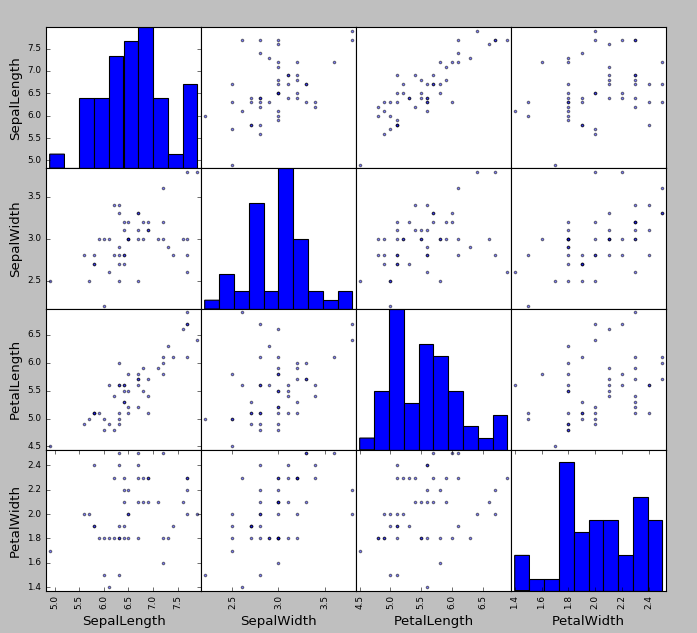
Attention
It only looks bad because I used the default colors. Plots can be customized to your liking!
Of course, there is a lot more to Pandas than solving simple tasks like this.
Pandas datatypes
Pandas provides a couple of very useful datatypes, Series and DataFrame:
Seriesrepresents 1D data, like time series, calendars, the output of one-variable functions, etc.DataFramerepresents 2D data, like a column-separated-values (CSV) file, a microarray, a database table, a matrix, etc.
A DataFrame is composed of multiple Series. More specifically, each
column of a DataFrame is a Series. That’s why we will see how the
Series datatype works first.
Attention
Most of what we will say about Series also applies to DataFrame‘s.
The similarities include how indexing is done, how broadcasting applies
to arithmetical operators and Boolean masks, how to compute statistics,
how to deal with missing values (nan‘s) and how plotting is done.
Pandas: Series
A Series is a one-dimensional array with a labeled axis. It can hold
arbitrary objects. It works a little like a list and a little like a
dict.
The axis is called the index, and can be used to access the elements; it is
very flexible, and not necessarily numerical.
To access the online documentation, type:
>>> s = pd.Series()
>>> help(s)
Creating a Series
Use the Series() constructor to create a new Series object, as follows.
When creating a Series, you can either specify both the date and the
index, like this:
>>> s = pd.Series(["a", "b", "c"], index=[2, 5, 8])
>>> s
2    a
5    b
8    c
dtype: object
>>> s.index
Int64Index([2, 5, 8], dtype='int64')
or pass a single dict in, in which case the index is built from the
dictionary keys:
>>> s = pd.Series({"a": "A", "b": "B", "c": "C"})
>>> s
a    A
b    B
c    C
dtype: object
>>> s.index
Index([u'a', u'b', u'c'], dtype='object')
or skip the index altogether: in this case, the default index (i.e. a
numerical index starting from 0) is automatically assigned:
>>> s = pd.Series(["a", "b", "c"])
>>> s
0    a
1    b
2    c
dtype: object
>>> s.index
RangeIndex(start=0, stop=3, step=1)
Finally, if given a single scalar (e.g. an int), the Series constructor
will replicate it for all indices:
>>> s = pd.Series(3, index=range(10))
>>> s
0    3
1    3
2    3
3    3
4    3
5    3
6    3
7    3
8    3
9    3
dtype: int64
Note
The type of the index changes in the previous exercises.
The library uses different types of index for performance reasons. The
Series class however works (more or less) the same in all cases, so
you can ignore these differences in practical applications.
Accessing a Series
Let’s create a Series representing the hours of sleep we had the chance to
get each day of the past week:
>>> sleephours = [6, 2, 8, 5, 9]
>>> days = ["mon", "tue", "wed", "thu", "fri"]
>>> s = pd.Series(sleephours, index=days)
>>> s
mon    6
tue    2
wed    8
thu    5
fri    9
dtype: int64
Now we can access the various elements of the Series both by their label
(i.e. the index) like we would with a dict:
>>> s["mon"]
6
as well as by their position, like we would with a list:
>>> s[0]
6
Warning
If the label or position is wrong, you get either a KeyError:
>>> s["sat"]
KeyError: 'sat'
or an IndexError:
>>> s[9]
IndexError: index out of bounds
We can also slice the positions, like we would with a list:
>>> s[-3:]
wed    8
thu    5
fri    9
dtype: int64
Note that both the data and the index are extracted correctly. It also works with labels:
>>> s["tue":"thu"]
tue    2
wed    8
thu    5
dtype: int64
The first and last n elements can be extracted also using head() and
tail():
>>> s.head(2)
mon    6
tue    2
dtype: int64
>>> s.tail(3)
wed    8
thu    5
fri    9
dtype: int64
Most importantly, can also explicitly pass in a list of positions, like this:
>>> s[[0, 1, 2]]
mon    6
tue    2
wed    8
dtype: int64
>>> s[["mon", "wed", "fri"]]
mon    6
wed    8
fri    9
dtype: int64

>>> s.head()
Warning
Passing in a tuple of positions does not work!
Operator Broadcasting
The Series class automatically broadcasts arithmetical operations by a
scalar to all of the elements. Consider adding 1 to our Series:
>>> s
mon    6
tue    2
wed    8
thu    5
fri    9
dtype: int64
>>> s + 1
mon     7
tue     3
wed     9
thu     6
fri    10
dtype: int64
As you can see, the addition was applied to all the entries! This also applies to multiplication and other arithmetical operations:
>>> s * 2
mon    12
tue     4
wed    16
thu    10
fri    18
dtype: int64
This is extremely useful: it frees the analyst from having to write loops. The (worse) alternative the above would be:
for x in s.index:
    s[x] += 1
which is definitely more verbose and error-prone, and also takes more time to execute!
Note
The concept of operator broadcasting was taken from the numpy
library, and is one of the key features for writing efficient,
clean numerical code in Python.
In a way, it is a “generalized” version of scalar products (from linear algebra).
The rules govering how broadcasting is applied can be pretty complex (and confusing). Here we will cover constant broadcasting only.
Masks and Filtering
Most importantly, broadcasting also applies to conditions:
>>> s > 6
mon     True
tue    False
wed     True
thu    False
fri     True
dtype: bool
Here the result is a Series with the same index as the original (that is,
the very same labels), and each label label is associated to the result of
the comparison s[label] > 6. This kind of series is called a mask.
Is it useful in any way?
Yes, of course! Masks can be used to filter the elements of a Series
according to a given condition:
>>> s[s > 6]
mon     7
wed     9
fri    10
dtype: int64
Here only those entries corresponding to True‘s in the mask have been
kept. For extracting the elements that satisfy the opposite of the condition,
write:
>>> s[s <= 6]
tue    3
thu    6
dtype: int64
or:
>>> s[~(s > 6)]
tue    3
thu    6
dtype: int64
The latter version is useful when the condition you are checking for is complex and can not be inverted easily.
Automatic Label Alignment
Operations between multiple time series are automatically aligned by label, meaning that elements with the same label are matched prior to carrying out the operation.
Consider this example:
>>> s[1:] + s[:-1]
fri     NaN         # <-- not common
mon     NaN         # <-- not common
thu    10.0         # <-- common element
tue     4.0         # <-- common element
wed    16.0         # <-- common element
dtype: float64
As you can see, the elements are summed in the right order! But what’s up with
those nan‘s?
The index of the resulting Series is the union of the indices of
the operands. What happens depend on whether a given label appears in both
ipnut Series or not:
- For common labels (in our case
"tue","wed","thu"), the outputSeriescontains the sum of the aligned elements. - For labels appearing in only one of the operands (
"mon"and"fri"), the result is anan, i.e. not-a-number.
Warning
nan means not a number.
It is just a symbolic constant that specifies that the object is a number-like entity with an invalid or undefined value. Think for instance of the result of division by 0.
In the example above, the result is a nan because it represents the
sum of an element, like s[1:]["fri"], and a non-existing element,
like s[:-1]["fro"].
It is used to indicate undefined results (like above) or missing measurements (as we will see).
The actual value of the nan symbol is taken from numpy, see
numpy.nan. You can actually use it to insert nan‘s manually:
>>> s["fri"] = np.nan
>>> s
mon    6.0
tue    2.0
wed    8.0
thu    5.0
fri    NaN
dtype: float64
Dealing with Missing Data
By default, missing entries and invalid results in Pandas are defined as
nan. Consider the Series from the previous example:
>>> t = s[1:] + s[:-1]
>>> t
fri     NaN
mon     NaN
thu    12.0
tue     6.0
wed    18.0
dtype: float64
There are different strategies for dealing with nan‘s. There is no “best”
strategy: you have to pick one depending on the problem you are trying to
solve.
Drop all entries that have a
nan, withdropna()(read it as drop N/A, i.e. not available):>>> nonan_t = t.dropna() >>> nonan_t thu 12.0 tue 6.0 wed 18.0 dtype: float64
Filling in the
nanentries with a more palatable value, for instance a default value that does not disrupt your statistics:>>> t.fillna(0.0) fri 0.0 mon 0.0 thu 12.0 tue 6.0 wed 18.0 dtype: float64
or:
>>> t.fillna("unknown")
fri    unknown
mon    unknown
thu         12
tue          6
wed         18
dtype: object
Filing in the
nanby imputing the missing value from the surrouding ones.>>> s mon NaN tue 2.0 wed 8.0 thu NaN fri NaN dtype: float64 >>> s.ffill() mon NaN tue 2.0 wed 8.0 thu 8.0 fri 8.0 dtype: float64
Warning
Most of Pandas function gracefully deal with missing values.
For instance the mean() method has a skipna argument can be either
True or False. If it is True, the mean will not consider the
missing values; if it is False, the result of a series containing
a nan will itself be a nan (as should happen in purely mathematical
terms).
Computing Statistics
Series objects support a variety of mathematical and statistical
operations:
The sum and product of all values in the
Series>>> s.sum() 30 >>> s.prod() 11340
The cumulative sum:
>>> s.cumsum()
mon     6
tue     8
wed    16
thu    21
fri    30
dtype: int64
The minimum and maximum values and their indices:
>>> s.max()
9
>>> s.argmax()
'fri'
>>> s[s.argmax()]
9
and the same for
s.min()ands.argmin().The mean, variance, std. deviation, median, quantiles, etc.:
>>> s.mean()
6.0
>>> s.var()
7.5
>>> s.std()
2.7386127875258306
>>> s.median()
6.0
>>> s.quantile([0.25, 0.5, 0.75])
0.25    6.0
0.50    7.0
0.75    9.0
dtype: float64
These can be paired with masks for awesome extraction effects:
>>> s[s > s.quantile(0.66)]
wed     9
fri    10
dtype: int64
The Pearson, Kendall, Spearman correlations between series:
>>> s.corr(s) # Pearson by default
1.0
>>> s.corr(s, method="spearman")
0.99999999999999989
The autocorrelation with arbitrary time lag:
>>> s.autocorr(lag=0)
1.0
>>> s.autocorr(lag=1)
-0.54812812776251907
>>> s.autocorr(lag=2)
0.99587059488582252
... and many, many others.
Note
A quick way to examine a Series is to use the describe() method:
>>> s.describe()
count     5.000000
mean      7.000000
std       2.738613
min       3.000000
25%       6.000000
50%       7.000000
75%       9.000000
max      10.000000
dtype: float64
Warning
You are not required to remember all these methods!
Just be aware that if you need basic statistical tool, probably pandas
has them.
Plotting
We want to visualize our simple sleeping hours data:
>>> sleephours = [6, 2, 8, 5, 9]
>>> days = ["mon", "tue", "wed", "thu", "fri"]
>>> s = pd.Series(sleephours, index=days)
Now that we have a Series, let’s import the additional matplotlib
module:
>>> import matplotlib.pyplot as plt
This is the customary idiom to import the library. Let’s plot the data!
With a simple line plot:
>>> s.plot()
>>> plt.show()
With a more readable bar plot:
>>> s.plot(kind="bar")
>>> plt.show()
With a histogram:
>>> s.plot(kind="hist")
>>> plt.show()
Note
There are very many ways to improve the looks of your plots, like changing the shape, size, margins, colors, labels, etc.
Browse the documentation for inspiration:
Note
To save the plot to a file instead of merely showing it on screen, use the
savefig() method of the matplotlib library:
>>> plt.savefig("output.png")
Pandas: DataFrame
Pandas DataFrame is the 2D analogue of a Series: it is essentially a
table of heterogeneous objects.
Recall that a Series holds both the values and the labels of all its
elements. Analogously, a DataFrame two major attributes:
- the
index, which holds the labels of the rows - the
columns, which holds the labels of the columns - the
shape, which describes the dimension of the table
Each column in the DataFrame is a Series: when you extract a column
from a DataFrame you get a proper Series, and you can operate on it
using all the tools presented in the previous section.
Further, most of the operations that you can do on a Series, you can also
do on an entire DataFrame. The sample principles apply: broadcasting, label
alignment, and plotting. They all work very similarly.
Warning
Not all operations work exactly the same on the two datatypes.
This is of course because some operations that make sense on a 2D table, do not really apply to a 1D sequence, and vice versa.
However the analogy holds well enough in most cases.
Creating a DataFrame
Just like for Series, there are various options. We can:
Create a
DataFramefrom a dictionary ofSeries:>>> d = { ... "name": ... pd.Series(["bobby", "ronald", "ronald", "ronald"]), ... "surname": ... pd.Series(["fisher", "fisher", "reagan", "mcdonald"]), ... } >>> df = pd.DataFrame(d) >>> df name surname 0 bobby fisher 1 ronald fisher 2 ronald reagan 3 ronald mcdonald >>> df.columns Index([u'name', u'surname'], dtype='object') >>> df.index RangeIndex(start=0, stop=4, step=1)
As you can see:
- the keys of the dictionary became the
columnsofdf - the
indexof the variousSeriesbecame theindexofdf.
Warning
If the
indexof the inputSeriesdo not match, since label alignment applies, the missing values are treated asnan‘s.This is exactly what happens in this example:
>>> d = {
>>>     "name":
>>>         pd.Series([0, 0], index=["a", "b"]),
>>>     "surname":
>>>         pd.Series([0, 0], index=["c", "d"]),
>>> }
>>> df = pd.DataFrame(d)
>>> df
name  surname
a   0.0      NaN
b   0.0      NaN
c   NaN      0.0
d   NaN      0.0
>>> df.columns
Index(['name', 'surname'], dtype='object')
>>> df.index
Index(['a', 'b', 'c', 'd'], dtype='object')
- the keys of the dictionary became the
Create a
DataFramefrom a single dictionary:>>> d = { ... "column1": [1., 2., 6., -1.], ... "column2": [0., 1., -2., 4.], ... } >>> df = pd.DataFrame(d) >>> df column1 column2 0 1.0 0.0 1 2.0 1.0 2 6.0 -2.0 3 -1.0 4.0
Again, the
columnsare taken from the keys, while theindexis set to the default one (i.e.range(0, num_rows)).A custom
indexcan be specified the usual way:>>> df = pd.DataFrame(d, index=["a", "b", "c", "d"]) >>> df column1 column2 a 1.0 0.0 b 2.0 1.0 c 6.0 -2.0 d -1.0 4.0
Create a
DataFramefrom a list of dictionaries:>>> data = [ ... {"a": 1, "b": 2}, ... {"a": 2, "c": 3}, ... ] >>> df = pd.DataFrame(data) >>> df a b c 0 1 2.0 NaN 1 2 NaN 3.0
Here the
columnsare taken (again) from the keys of the dictionaries, while theindexis the default one. Since not all common keys appear in all input dictionaries, missing values (i.e.nan‘s) are automatically added todf.
Note
Once a DataFrame has been created, you can change interactively its
index and columns:
>>> d = {
...     "column1": [1., 2., 6., -1.],
...     "column2": [0., 1., -2., 4.],
... }
>>> df = pd.DataFrame(d)
>>> df
column1  column2
0      1.0      0.0
1      2.0      1.0
2      6.0     -2.0
3     -1.0      4.0
>>> df.columns = ["bar", "bar"]
>>> df.columns
Index([u'foo', u'bar'], dtype='object')
>>> df.index = range(df.shape[1])
>>> df.index
Int64Index([0, 1, 2, 3], dtype='int64', length=4)
Loading a CSV file
Of course, the advantage of Pandas is that it allows to load data from many different file formats. Here we will only consider CSV (comma separated values) files and similar.
To load a CSV into a DataFrame, for instance the iris dataset, type:
>>> df = pd.read_csv("iris.csv")
>>> print type(df)
<class 'pandas.core.frame.DataFrame'>
Now that it’s loaded, let’s print some information about it:
>>> df.columns
Index([u'SepalLength', u'SepalWidth', u'PetalLength', u'PetalWidth', u'Name'], dtype='object')
>>> df.index
RangeIndex(start=0, stop=150, step=1)
>>> df.shape
(150, 5)
>>> print df
...
Note
The CSV file format is not really well-defined.
This means that the CSV files that you’ll encounter in the wild can (and probably will!) be very different from one another.
Given the diversity of this (under-specified) file format, the
read_csv() provides a large number of options to deal with many
of the (otherwise code-breaking) differences between CSV-like files.
Here is an excerpt from the read_csv() manual:
>>> help(pd.read_csv)

Help on function read_csv in module pandas.io.parsers:

read_csv(filepath_or_buffer, sep=',', delimiter=None, header='infer',
    names=None, index_col=None, usecols=None, squeeze=False,
    prefix=None, mangle_dupe_cols=True, dtype=None, engine=None,
    converters=None, true_values=None, false_values=None,
    skipinitialspace=False, skiprows=None, nrows=None, na_values=None,
    keep_default_na=True, na_filter=True, verbose=False,
    skip_blank_lines=True, parse_dates=False,
    infer_datetime_format=False, keep_date_col=False, date_parser=None,
    dayfirst=False, iterator=False, chunksize=None,
    compression='infer', thousands=None, decimal='.',
    lineterminator=None, quotechar='"', quoting=0, escapechar=None,
    comment=None, encoding=None, dialect=None, tupleize_cols=False,
    error_bad_lines=True, warn_bad_lines=True, skipfooter=0,
    skip_footer=0, doublequote=True, delim_whitespace=False,
    as_recarray=False, compact_ints=False, use_unsigned=False,
    low_memory=True, buffer_lines=None, memory_map=False,
    float_precision=None)

Read CSV (comma-separated) file into DataFrame

Also supports optionally iterating or breaking of the file
into chunks.

Additional help can be found in the `online docs for IO Tools
<http://pandas.pydata.org/pandas-docs/stable/io.html>`_.
As you can see, you can tweak the read_csv() method in very many
ways, in order to make it load your data the proper way.
Note
A similar function esists for reading Excel files, read_excel().
Example: A malformed TSV file. Let’s load a TAB-separated file instead (i.e. a CSV file that uses TABs instead of commas). The file can be found here:
It describes a mapping from UniProt protein IDs (i.e. sequences) to hits in the Protein Data Bank (i.e. structures). The TSV file looks like this:
# 2014/07/08 - 14:59
SP_PRIMARY  PDB
A0A011      3vk5;3vka;3vkb;3vkc;3vkd
A0A2Y1      2jrd
A0A585      4mnq
A0A5B4      2ij0
A0A5B9      2bnq;2eyr;2eys;2eyt;3kxf;3o6f;3o8x;3o9w;3qux;3t0e;3ta3;3tvm
A0A5E3      1hq4;1ob1
A0AEF5      4iu2;4iu3
A0AEF6      4iu2;4iu3
A0AQQ7      2ib5
Note that the two columns are separated by a TAB. Note also that the first row is actually a comment.
We can use the sep (separator) argument of the read_csv() function
to take care of the TABs. Let’s write:
>>> df = pd.read_csv("uniprot_pdb.tsv", sep="\t")
>>> df.shape
(33637, 1)
>>> df.columns
Index([u'# 2014/07/08 - 14:59'], dtype='object')
>>> df.head()
# 2014/07/08 - 14:59
SP_PRIMARY                       PDB
A0A011      3vk5;3vka;3vkb;3vkc;3vkd
A0A2Y1                          2jrd
A0A585                          4mnq
A0A5B4                          2ij0
>>> df.head().shape
(5, 1)
Unfortunately, the shape of the DataFrame is wrong: there is only one
column!
The problem is that the very first line (the comment) contains no tabs: this makes Panda think that there is only one column.
We have to tell read_csv() to either ignore the first line:
>>> df = pd.read_csv("uniprot_pdb.tsv", sep="\t", skiprows=1)
>>> df.shape
(33636, 2)
>>> df.head()
SP_PRIMARY                                                PDB
0     A0A011                           3vk5;3vka;3vkb;3vkc;3vkd
1     A0A2Y1                                               2jrd
2     A0A585                                               4mnq
3     A0A5B4                                               2ij0
4     A0A5B9  2bnq;2eyr;2eys;2eyt;3kxf;3o6f;3o8x;3o9w;3qux;3...
>>> df.shape
(33636, 2)
or, as an alternative, to ignore all comment lines, i.e. all lines that start
with a sharp "#" character:
>>> df = pd.read_csv("uniprot_pdb.tsv", sep="\t", comment="#")
>>> df.shape
(33636, 2)
>>> df.head()
SP_PRIMARY                                                PDB
0     A0A011                           3vk5;3vka;3vkb;3vkc;3vkd
1     A0A2Y1                                               2jrd
2     A0A585                                               4mnq
3     A0A5B4                                               2ij0
4     A0A5B9  2bnq;2eyr;2eys;2eyt;3kxf;3o6f;3o8x;3o9w;3qux;3...
>>> df.head().shape
(5, 2)
Now the number of columns is correct!
Example: microarray data. Let’s also try to load the microarray file in Stanford PCL format (namely, a disguised TAB-separated-values file) available here:
Again, it is pretty easy:
>>> df = pd.read_csv("2010.DNAdamage.pcl", sep="\t")
>>> df.shape
(6128, 55)
>>> df.columns
Index([u'YORF', u'NAME', u'GWEIGHT', u'wildtype + 0.02% MMS (5 min)',
u'wildtype + 0.02% MMS (15 min)', u'wildtype + 0.02% MMS (30 min)',
u'wildtype + 0.2% MMS (45 min)', u'wildtype + 0.02% MMS (60 min)',
u'wildtype + 0.02% MMS (90 min)', u'wildtype + 0.02% MMS (120 min)',
u'mec1 mutant + 0.02% MMS (5 min)', u'mec1 mutant + 0.02% MMS (15 min)',
u'mec1 mutant + 0.02% MMS (30 min)',
u'mec1 mutant + 0.02% MMS (45 min)',
u'mec1 mutant + 0.02% MMS (60 min)',
u'mec1 mutant + 0.02% MMS (90 min)',
u'mec1 mutant + 0.02% MMS (120 min)',
u'dun1 mutant + 0.02% MMS (30 min)',
u'dun1 mutant + 0.02% MMS (90 min)',
u'dun1 mutant + 0.02% MMS (120 min)',
u'wildtype + gamma irradiation (5 min)',
u'wildtype + gamma irradiation (10 min)',
...
u'crt1 mutant vs wild type (expt 1)',
u'crt1 mutant vs. wild type (expt 2)',
u'GAL-inducible ROX1 on galactose'],
dtype='object')
Warning
... at least at a quick glance.
Additional care must be taken for this data: some columns are not
separated correctly (just look at the file with the less command
to see what I mean).
Feel free to try and improve the example above to properly load the microarray file!
Extracting Rows and Columns
Row and column extraction from a DataFrame can be very easy to very
complex, depending on what you want to do.
Here we will only deal with elementary extraction methods.
Note
If you wish to know more, especially about the ever useful ix attribute,
take a look at the documentation:
The (non-exhaustive) list of alternatives is:
| Operation | Syntax | Result |
|---|---|---|
| Select column | df[col] |
Series |
| Select row by label | df.loc[label] |
Series |
| Select row by integer location | df.iloc[loc] |
Series |
| Slice rows | df[5:10] |
DataFrame |
| Select rows by boolean vector | df[bool_vec] |
DataFrame |
Note
For simplicity, in the following examples we will use a random sample taken from the iris dataset, computed like this:
>>> import numpy as np
>>> import pandas as pd
>>> np.random.seed(0)
>>> df = pd.read_csv("iris.csv")
>>> small = df.iloc[np.random.permutation(df.shape[0])].head()
>>> small.shape
(5, 5)
>>> small
SepalLength  SepalWidth  PetalLength  PetalWidth             Name
114          5.8         2.8          5.1         2.4   Iris-virginica
62           6.0         2.2          4.0         1.0  Iris-versicolor
33           5.5         4.2          1.4         0.2      Iris-setosa
107          7.3         2.9          6.3         1.8   Iris-virginica
7            5.0         3.4          1.5         0.2      Iris-setosa
Brief explanation: here we use numpy.random.permutation() to generate
a random permutation of the indices from 0 to df.shape[0], i.e.
the number of rows in the iris dataset; then we use these random
numbers as row indices to permute all the rows in df; finally, we
take the first 5 rows of the permuted df using the head()
method.
A
DataFramecan now be accessed like a regular dictionary to extract individual columns – indeed, you can also print its keys!:>>> small.columns Index([u'SepalLength', u'SepalWidth', u'PetalLength', u'PetalWidth', u'Name'], dtype='object') >>> small.keys() Index([u'SepalLength', u'SepalWidth', u'PetalLength', u'PetalWidth', u'Name'], dtype='object')
Now we access
smallby column name; the result is aSeries:>>> type(small["Name"]) <class 'pandas.core.series.Series'> >>> small["Name"] 114 Iris-virginica 62 Iris-versicolor 33 Iris-setosa 107 Iris-virginica 7 Iris-setosa Name: Name, dtype: object
If the name of the column is compatible with the Python conventions for variable names, you can also treat columns as if they were actual attributes of the
dfobject:>>> small.Name 114 Iris-virginica 62 Iris-versicolor 33 Iris-setosa 107 Iris-virginica 7 Iris-setosa Name: Name, dtype: object
Warning
Here
Nameis a variable created on-the-fly by Pandas when loading the iris setosa dataset!It is possible to extract multiple columns in one go; the result will be a
DataFrame:>>> small[["SepalLength", "PetalLength"]] SepalLength PetalLength 114 5.8 5.1 62 6.0 4.0 33 5.5 1.4 107 7.3 6.3 7 5.0 1.5
Warning
Note that the order of the column labels matters!
Compare this with the previous code fragment:
>>> small[["PetalLength", "SepalLength"]]
PetalLength  SepalLength
114          5.1          5.8
62           4.0          6.0
33           1.4          5.5
107          6.3          7.3
7            1.5          5.0
To extract the rows, we can use the
locandilocattributes:locallows to retrieve a row by label:>>> small.loc[114] SepalLength 5.8 SepalWidth 2.8 PetalLength 5.1 PetalWidth 2.4 Name Iris-virginica Name: 114, dtype: object >>> type(small.loc[114]) <class 'pandas.core.series.Series'>
The result is a
Series.ilocallows to retrieve a row by position:>>> small.iloc[0] SepalLength 5.8 SepalWidth 2.8 PetalLength 5.1 PetalWidth 2.4 Name Iris-virginica Name: 114, dtype: object
The result is, again, a
Series.The
locandilocattribute also allow to retrieve multiple rows:>>> small.loc[[114,7,62]] SepalLength SepalWidth PetalLength PetalWidth Name 114 5.8 2.8 5.1 2.4 Iris-virginica 7 5.0 3.4 1.5 0.2 Iris-setosa 62 6.0 2.2 4.0 1.0 Iris-versicolor >>> small.iloc[[0,1,2]] SepalLength SepalWidth PetalLength PetalWidth Name 114 5.8 2.8 5.1 2.4 Iris-virginica 62 6.0 2.2 4.0 1.0 Iris-versicolor 33 5.5 4.2 1.4 0.2 Iris-setosa
This time, the result is a
DataFrame.Warning
Again, note that the order of the row labels matters!
Broadcasting, Masking, Label Alignment
All of these work just like with Series:
Broacasting is applied automatically to all rows:
>>> small["SepalLength"] + small["SepalWidth"]
114     8.6
62      8.2
33      9.7
107    10.2
7       8.4
dtype: float64
or to the whole table:
>>> small + small
     SepalLength  SepalWidth  PetalLength  PetalWidth  \
114         11.6         5.6         10.2         4.8
62          12.0         4.4          8.0         2.0
33          11.0         8.4          2.8         0.4
107         14.6         5.8         12.6         3.6
7           10.0         6.8          3.0         0.4

                               Name
114    Iris-virginicaIris-virginica
62   Iris-versicolorIris-versicolor
33           Iris-setosaIris-setosa
107    Iris-virginicaIris-virginica
7            Iris-setosaIris-setosa
The usual label alignment (and corresponding mismatching-labels-equals-
nan) rules apply:>>> small["SepalLength"][1:] + small["SepalWidth"][:-1] 7 NaN 33 9.7 62 8.2 107 10.2 114 NaN dtype: float64
Warning
Both row labels and column labels are automatically aligned!
Masking works as well, for instance:
>>> small.PetalLength[small.PetalLength > 5]
114    5.1
107    6.3
Name: PetalLength, dtype: float64

>>> small["PetalLength"][small["PetalLength"] > 5]
114    5.1
107    6.3
Name: PetalLength, dtype: float64

>>> small["Name"][small["PetalLength"] > 5]
114    Iris-virginica
107    Iris-virginica
Name: Name, dtype: object

>>> small[["Name", "PetalLength", "SepalLength"]][small.Name == "Iris-virginica"]
               Name  PetalLength  SepalLength
114  Iris-virginica          5.1          5.8
107  Iris-virginica          6.3          7.3
Statistics can be computed on rows:
>>> df.loc[114][:-1].mean()
4.0249999999999995
(Here the
[:-1]skips over theNamecolumn), on columns:>>> df.PetalLength.mean() 3.7586666666666662 >>> df["PetalLength"].mean() 3.7586666666666662
or on the whole table:
>>> df.mean()
SepalLength    5.843333
SepalWidth     3.054000
PetalLength    3.758667
PetalWidth     1.198667
dtype: float64
or between rows:
>>> small.PetalLength.cov(small.SepalLength)
1.6084999999999996
You can combine them with masking as well:
>>> small[["Name", "PetalLength", "SepalLength"]][small.PetalLength > small.PetalLength.mean()]
                Name  PetalLength  SepalLength
114   Iris-virginica          5.1          5.8
62   Iris-versicolor          4.0          6.0
107   Iris-virginica          6.3          7.3
Merging Tables
Merging different dataframes is performed using the merge() function.
Merging means that, given two tables with a common column name, first the rows with the same column value are matched; then a new table is created by concatenating the matching rows.
Here is an explanatory image:
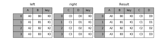
(Taken from the Merge, join, and concatenate section of the official Pandas documentation.)
Note
Only the column name must be the same in both tables: the actual values in the column may differ.
What happens when the column values are different, depends on the
how argument of the merge() function. See below.
A simple example of merging two tables describing protein properties (appropriately simplified for ease of exposition):
sequences = pd.DataFrame({
    "id":  ["Q99697", "O18400", "P78337", "Q9W5Z2"],
    "seq": ["METNCR", "MDRSSA", "MDAFKG", "MTSMKD"],
})

names = pd.DataFrame({
    "id":   ["Q99697", "O18400", "P78337", "P59583"],
    "name": ["PITX2_HUMAN", "PITX_DROME",
             "PITX1_HUMAN", "WRK32_ARATH"],
})

print "input dataframes:"
print sequences
print names

print "full inner:"
print pd.merge(sequences, names, on="id", how="inner")

print "full left:"
print pd.merge(sequences, names, on="id", how="left")

print "full right:"
print pd.merge(sequences, names, on="id", how="right")

print "full outer:"
print pd.merge(sequences, names, on="id", how="outer")
Note that the "id" column appears in both dataframes. However, the values
in the column differ: "Q9W5Z2" only appears in the sequences table,
while "P59583" only appears in names.
Let’s see what happens using the four different joining semantics:
input dataframes:
id     seq
 0  Q99697  METNCR
 1  O18400  MDRSSA
 2  P78337  MDAFKG
 3  Q9W5Z2  MTSMKD

id         name
 0  Q99697  PITX2_HUMAN
 1  O18400   PITX_DROME
 2  P78337  PITX1_HUMAN
 3  P59583  WRK32_ARATH

# mismatched ids are dropped
full inner:
id     seq         name
 0  Q99697  METNCR  PITX2_HUMAN
 1  O18400  MDRSSA   PITX_DROME
 2  P78337  MDAFKG  PITX1_HUMAN

# ids are taken from the left table
full left:
id     seq         name
 0  Q99697  METNCR  PITX2_HUMAN
 1  O18400  MDRSSA   PITX_DROME
 2  P78337  MDAFKG  PITX1_HUMAN
 3  Q9W5Z2  MTSMKD          NaN

# ids are taken from the right table
full right:
id     seq         name
 0  Q99697  METNCR  PITX2_HUMAN
 1  O18400  MDRSSA   PITX_DROME
 2  P78337  MDAFKG  PITX1_HUMAN
 3  P59583     NaN  WRK32_ARATH

# all ids are retained
full outer:
id     seq         name
 0  Q99697  METNCR  PITX2_HUMAN
 1  O18400  MDRSSA   PITX_DROME
 2  P78337  MDAFKG  PITX1_HUMAN
 3  Q9W5Z2  MTSMKD          NaN
 4  P59583     NaN  WRK32_ARATH
To summarize, the how argument establishes the semantics for the mismatched
labels, and where the nan‘s should be inserted.
Example. Dataframe merging automatically takes care of replicating rows appropriately if the same key appears twice.
For instance, consider this code:
sequences = pd.DataFrame({
    "id":  ["Q99697", "Q99697"],
    "seq": ["METNCR", "METNCR"],
})

names = pd.DataFrame({
    "id":   ["Q99697", "O18400", "P78337", "P59583"],
    "name": ["PITX2_HUMAN", "PITX_DROME",
             "PITX1_HUMAN", "WRK32_ARATH"],
})

print "input dataframes:"
print sequences
print names

print "full:"
print pd.merge(sequences, names, on="id", how="inner")
The result is:
input dataframes:
id     seq
 0  Q99697  METNCR
 1  Q99697  METNCR

id         name
 0  Q99697  PITX2_HUMAN
 1  O18400   PITX_DROME
 2  P78337  PITX1_HUMAN
 3  P59583  WRK32_ARATH

full:
id     seq         name
 0  Q99697  METNCR  PITX2_HUMAN
 1  Q99697  METNCR  PITX2_HUMAN
As you can see, rows are replicated appropriately!
Hint
This is extremely useful.
Consider for instance the problem of having to compute statistics on all the three gene-exon-CDS tables in the exercises section, jointly.
Using merge() it is easy to merge the three tables in a single, big
table, where the gene information is appropriately replicated for all
gene exons, and the exon information is replicated for all coding
sequences!
Note
The merge() method also allows to join tables by more than one column,
using the key attribute. See the official documentation here:
Grouping Tables
The groupby method is essential for efficiently performing operations on
groups of rows – especially split-apply-aggregate operations.
A picture is worth one thousand words, so here it is:
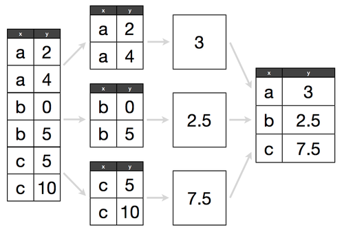
(Picture source: Hadley Wickham’s Data Science in R slides)
The groupby() method allows to extract groups of rows with the same value
(the “split” part), perform some computation on them (the “apply” part) and
then combine the results into a single table over the groups (the “aggregate”
part).
Example. Let’s take the iris dataset. We want to compute the average of the four data tables for the three different iris species.
The result should be a 3 species (rows) by 4 columns (petal/sepal length/width) dataframe.
First, let’s load the CSV file and print some information:
>>> iris = pd.read_csv("iris.csv")
>>> iris.info()
<class 'pandas.core.frame.DataFrame'>
RangeIndex: 150 entries, 0 to 149
Data columns (total 5 columns):
SepalLength    150 non-null float64
SepalWidth     150 non-null float64
PetalLength    150 non-null float64
PetalWidth     150 non-null float64
Name           150 non-null object
dtypes: float64(4), object(1)
memory usage: 5.9+ KB
Here is how to do that with groupby(). First, let’s group all rows of the
dataframe by the Name column:
>>> grouped = iris.groupby(iris.Name)
>>> type(grouped)
<class 'pandas.core.groupby.DataFrameGroupBy'>
>>> for group in grouped:
...     print group[0], group[1].shape
...
Iris-setosa (50, 5)
Iris-versicolor (50, 5)
Iris-virginica (50, 5)
The groupby method returns a pandas.DataFrameGroupBy object (the
details are not important).
- To select a single group, write::
>>> group_df = grouped.get_group("Iris-versicolor")
>>> print type(group)
<class 'pandas.core.frame.DataFrame'>
>>> group.info()
Int64Index: 50 entries, 50 to 99
Data columns (total 5 columns):
SepalLength    50 non-null float64
SepalWidth     50 non-null float64
PetalLength    50 non-null float64
PetalWidth     50 non-null float64
Name           50 non-null object
dtypes: float64(4), object(1)
memory usage: 2.3+ KB
Note
As shown by the above code snippet, iterating over the grouped variable
returns (value-of-Name, DataFrame) tuples:
- The first element is the value of the column
Nameshared by the group - The second element is a
DataFrameincluding only the rows in that group.
The whole idea is that you can apply some transformation (e.g. mean()) to
the individual groups automatically, using the aggregate() method
directly on the grouped variable.
For instance, let’s compute the mean of all columns for the three groups:
>>> iris_mean_by_name = grouped.aggregate(pd.DataFrame.mean)
>>> iris_mean_by_name.info()
<class 'pandas.core.frame.DataFrame'>
Index: 3 entries, Iris-setosa to Iris-virginica
Data columns (total 4 columns):
SepalLength    3 non-null float64
SepalWidth     3 non-null float64
PetalLength    3 non-null float64
PetalWidth     3 non-null float64
dtypes: float64(4)
memory usage: 120.0+ bytes
So the result of aggregate() is a dataframe. Here is what it looks like:
>>> iris_mean_by_name
SepalLength  SepalWidth  PetalLength  PetalWidth
Name
Iris-setosa            5.006       3.418        1.464       0.244
Iris-versicolor        5.936       2.770        4.260       1.326
Iris-virginica         6.588       2.974        5.552       2.026
Warning
Note that the Name colum of the iris dataframe becomes the
index of the aggregated iris_mean_by_name dataframe: it is not a
proper column anymore!
The only actual columns are:
>>> iris_mean_by_name.columns
Index([u'SepalLength', u'SepalWidth', u'PetalLength', u'PetalWidth'], dtype='object')
Note
The groupby() method also allows to group by more than one column,
using the key attribute. See the official documentation here: