Numpy: a cursory overview
Warning
This is an appendix.
This material will not be part of the final exam.
Numpy is a freely available library for performing efficient numerical computations over scalars, vectors, matrices, and more generally N-dimensional tensors.
Its main features are:
- Flexible indexing and manipulation of arbitrary dimensional data.
- Many numerical routines (linear algebra, Fourier analysis, local and global optimization, etc.) using a variety of algorithms.
- Clean Python interface to many underlying libraries (for instance, the GNU Scientific Library, or GSL), which are used as efficient implementations of numerical algorithms.
- Support for random sampling from a variety of distributions.
This list is far from complete!
Documentation & Source
The official numpy website is:
The numpy source code is available at:
and is distributed under the numpy license:
Importing numpy
The customary idiom to import numpy is:
>>> import numpy as np
>>> help(np)
Importing specific sub-modules also makes sense, so feel free to write (in this case for the linear algebra module):
>>> import numpy.linalg as la
>>> help(la)
The Array class
An ndarray is what it says: an N-dimensional array (also known as a
tensor).
The usual concepts encountered in analysis and algebra can be implemented as arrays: vectors are 1D arrays, matrices are 2D arrays.
Given an array x, its dimensionality and type can be ascertained by
using the shape, ndim and dtype attributes:
>>> x = np.zeros(10)
array([ 0.,  0.,  0.,  0.,  0.,  0.,  0.,  0.,  0.,  0.])
>>> print type(x)
<type 'numpy.ndarray'>
>>> print x.shape
(10,)
>>> print x.ndim
1
>>> print x.dtype
float64
Creating an Array
Creating arrays from scratch can be useful to start off your mathematical code or for debugging purposes. A few useful creation functions are:
Creating an all-zero array is simple with
np.zeros():>>> # One dimensional case >>> x = np.zeros(2) >>> x array([ 0., 0.]) >>> # Two dimensional case >>> x = np.zeros((2, 2)) >>> x array([[ 0., 0.], [ 0., 0.]]) >>> x.shape (2, 2) >>> # Three dimensional case >>> x = np.zeros((2, 2, 2)) >>> x array([[[ 0., 0.], [ 0., 0.]], [[ 0., 0.], [ 0., 0.]]]) >>> x.shape (2, 2, 2)
Creating an all-ones array is equally simple with
np.ones():>>> # N-dimensional case >>> x = np.ones((2, 5, 5, 10)) >>> x.shape (2, 5, 5, 10)
To create a diagonal matrix, use either the
diag()andones()methods together, or theeye()method (reminiscent of Matlab):>>> np.diag(np.ones(3)) array([[ 1., 0., 0.], [ 0., 1., 0.], [ 0., 0., 1.]]) >>> np.eye(3) array([[ 1., 0., 0.], [ 0., 1., 0.], [ 0., 0., 1.]])
The numpy analogue of
range()isnp.arange():>>> x = np.arange(10) >>> x.shape (10,) >>> x array([0, 1, 2, 3, 4, 5, 6, 7, 8, 9])
Converting from an existing list or list-of-lists object:
>>> l = [range(3*i,3*(i+3),3) for i in range(3)]
>>> l
[[0, 3, 6], [3, 6, 9], [6, 9, 12]]
>>> np.array(l)
array([[ 0,  3,  6],
       [ 3,  6,  9],
       [ 6,  9, 12]])
In this case, the
dtypewill be based on the type of the elements in the inputlist.Random sampling an array from a distribution:
>>> # Sampling a single scalar from a real-valued uniform (sampling
>>> # functions return a scalar if no shape information is given)
>>> x = np.random.uniform(0, 10)
>>> x
3.9300397597884897

>>> # Sampling a 3-element vector from a Normal distribution
>>> # with mean=1 and sigma=0.2
>>> x = np.random.normal(1, 0.2, size=3)
>>> x
array([ 1.2001157 ,  0.94376082,  1.09514026])

>>> # Sampling a binary 3x3 matrix, i.e. from a uniform
>>> # distribution over integers
>>> x = np.random.randint(0, 2, size=(3, 3))
>>> x
array([[1, 0, 0],
       [1, 0, 1],
       [0, 1, 0]])
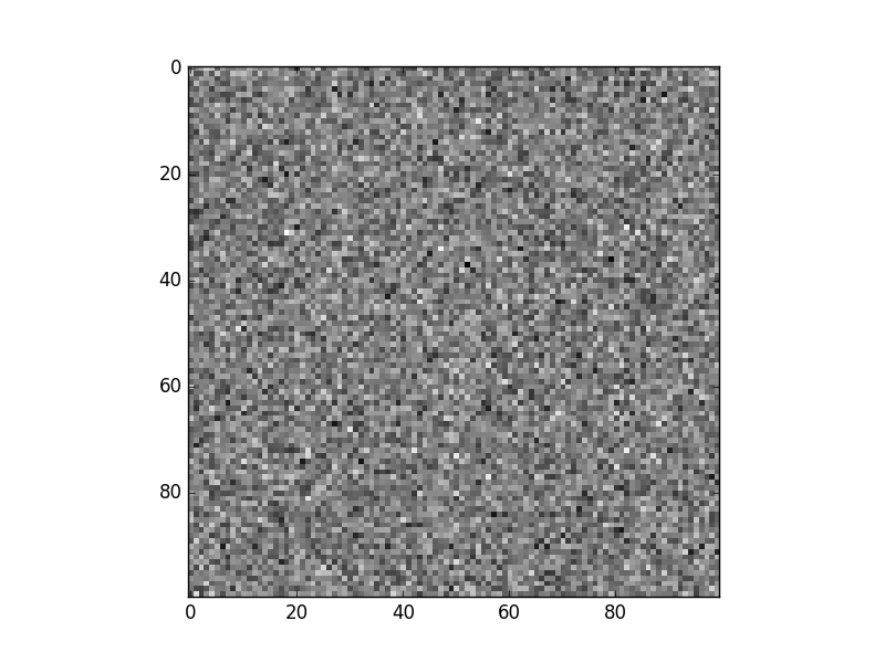
Example. To sample a random 100x100 matrix where every entry is distributed according to a normal distribution, write:
import numpy as np
import matplotlib.pyplot as plt

np.random.seed(0)

rm = np.random.normal(0, 1, size=(100, 100))

plt.imshow(rm, cmap="gray", interpolation="nearest")
plt.savefig("random-matrix.png")
The result is:
Note
The reference manual of the numpy.random module is here:
For a quick-and-dirty explanation of (pseudo!) random number generation as used in Computer Science, see:
The numpy.random RNG makes use of the very popular Mersenne Twister (MT)
PRNG. For an introduction, see here:
Warning
For reproducibility, make sure to initialize the pseudo-random number
generator with np.random.seed() before running your code, i.e.:
>>> np.random.seed(0)
After setting the seed, your code will be deterministic as long as calls to the sampling routines above remain the same.
From pandas to numpy and back
It is very easy to “convert” a Series or DataFrame into an array: as a
matter of facts, these Pandas types are built on numpy arrays: their
underlying array is accessible through the .values attribute.
(Pandas of course coats the underlying array with a lot of useful functionality!)
For instance, given a DataFrame of the iris dataset:
iris = pd.read_csv("iris.csv")
the underlying array can be accessed through its .values attribute:
>>> # For a table of two columns
>>> type(iris[["PetalLength", "SepalLength"]])
<class 'pandas.core.frame.DataFrame'>
>>> type(iris[["PetalLength", "SepalLength"]].values)
<type 'numpy.ndarray'>
The same can be done with individual Series objects, e.g. the columns
of the DataFrame:
>>> type(iris.PetalWidth.values)
<type 'numpy.ndarray'>
It is equally easy to construct a DataFrame out of an arrray: just call
the DataFrame passing it the array as an argument:
>>> pd.DataFrame(x)
   0  1  2
0  0  1  2
1  3  4  5
2  6  7  8
If you also want to assign the column and row labels, you can pass them as optional arguments:
>>> pd.DataFrame(x,
...              columns=['a', 'b', 'c'],
...              index=['one', 'two', 'three'])
       a  b  c
one    0  1  2
two    3  4  5
three  6  7  8
Reshaping
Reshaping. The arrangement of entries into rows, columns, tubes, etc. can be
changed at any time using the reshape() and ravel() methods:
>>> # Turn a 9-element vector into a 3x3 matrix
>>> x = np.arange(9)
>>> x
array([0, 1, 2, 3, 4, 5, 6, 7, 8])
>>> x.reshape((3, 3))
array([[0, 1, 2],
       [3, 4, 5],
       [6, 7, 8]])

>>> # Turn a 3x3 matrix into a 9-element vector
>>> x = np.ones((3, 3))
>>> x
array([[ 1.,  1.,  1.],
       [ 1.,  1.,  1.],
       [ 1.,  1.,  1.]])
>>> x.ravel()
array([ 1.,  1.,  1.,  1.,  1.,  1.,  1.,  1.,  1.])
Indexing
Given an array of shape (n1, n2, ..., nd), you can extract a single element
through its index.
For instance, in the 2D case:
>>> x = np.arange(9).reshape((3, 3))
>>> x
array([[0, 1, 2],
       [3, 4, 5],
       [6, 7, 8]])
>>> x[0,0]  # first row, first column
0
>>> x[1,2]  # second row, third column
5
>>> x[2,0]  # thrid row, first column
6
In the example above, x[i,j] extracts the element in row i, column
j – just like in standard matrix algebra.
You can also use the colon : notation to select specify all the elements
on an axis, for instance a whole column, a whole row, or an entire sub-array:
>>> # The first row
>>> x[0,:]
array([0, 1, 2])

>>> # A shorthand for the first row
>>> x[0]
array([0, 1, 2])

>>> # The first column (no shorthand available)
>>> x[:,1]
array([1, 4, 7])


>>> # A sub-table
>>> x[1:3, :]
array([[3, 4, 5],
       [6, 7, 8]])
The very same syntax applies to the general N-dimensional case:
>>> x = np.arange(10**5).reshape((10,)*5)
>>> x.shape
(10, 10, 10, 10, 10)
>>> x[1,2,3,4,5]
12345
>>> x[0,0,:,:,0]
array([[  0,  10,  20,  30,  40,  50,  60,  70,  80,  90],
       [100, 110, 120, 130, 140, 150, 160, 170, 180, 190],
       [200, 210, 220, 230, 240, 250, 260, 270, 280, 290],
       [300, 310, 320, 330, 340, 350, 360, 370, 380, 390],
       [400, 410, 420, 430, 440, 450, 460, 470, 480, 490],
       [500, 510, 520, 530, 540, 550, 560, 570, 580, 590],
       [600, 610, 620, 630, 640, 650, 660, 670, 680, 690],
       [700, 710, 720, 730, 740, 750, 760, 770, 780, 790],
       [800, 810, 820, 830, 840, 850, 860, 870, 880, 890],
       [900, 910, 920, 930, 940, 950, 960, 970, 980, 990]])
Note
It can be difficult to visualize operations over N-dimensional arrays, when N is larger than 3.
However, it is much easier when the axes have a concrete semantics. For
instance, assume that the 4D array performace holds the performance
of several sequence alignment algorithms over multiple sequence clusters
in multiple databases:
- The first axis is the index of the algorithm
- The second axis is the index of the database
- The third axis is the index of a cluster of sequences in the database
- The fourth axis is one of three measures of performance: precision, recall, and accuracy
Your tensor looks like this:
performances[alg][db][cluster][measure]
Then in extract the accuracy of algorithm 1 over all databases
and sequence clusters, you can just do:
performances[1,:,:,0]
or even:
performances[1,:,:,-1]
Now that the axes have a concrete semantics, it is much easier to see what this operation does!
Arithmetic and Functions
Operations between scalars and arrays are broadcast, like in Pandas (and more generally in linear algebra). For instance:
>>> x = np.arange(5)
>>> 10 * x
array([ 0, 10, 20, 30, 40])
>>> y = -x
>>> y
array([ 0, -10, -20, -30, -40])
Operations between equally-shaped arrays operate element-wise:
>>> x
array([0, 1, 2, 3, 4])
>>> x + x
array([0, 2, 4, 6, 8])
>>> x + y
array([0, 0, 0, 0, 0])
Operations can update the sub-arrays automatically:
>>> x = np.arange(16).reshape((4, 4))
>>> x
array([[ 0,  1,  2,  3],
       [ 4,  5,  6,  7],
       [ 8,  9, 10, 11],
       [12, 13, 14, 15]])
>>> x[1:3,1:3] += 100 # Note the automatic assignment!
>>> x
array([[  0,   1,   2,   3],
       [  4, 105, 106,   7],
       [  8, 109, 110,  11],
       [ 12,  13,  14,  15]])
Operations between arrays of different shapes but compatible sizes are
broadcast by “matching” the last (right-most) dimension. For instance,
addition between a matrix x and a vector y broadcasts y over all
rows of x:
>>> x = np.arange(9).reshape((3, 3))
>>> y = np.arange(3)
>>> x + y
array([[ 0,  2,  4],
       [ 3,  5,  7],
       [ 6,  8, 10]])
The result, x + y, can be seen as the result of:
result = np.zeros(x.shape)
for i in range(x.shape[0]):
    result[i,:] = x[i,:] + y[:]
As you can see, the last (right-most) dimension of x is matched to the last
(and only) dimension of y.
Warning
Operations between arrays of incompatible sizes raise an error:
>>> np.arange(3) + np.arange(2)
Traceback (most recent call last):
  File "<stdin>", line 1, in <module>
ValueError: operands could not be broadcast together with shapes (3,) (2,)
Mathematical Functions
Most of the usual mathematical functions are implemented in numpy, including the usual max and min operators and trigonometric functions.
For instance:
>>> np.sin(0), np.cos(0)
(0.0, 1.0)
>>> np.sin(np.pi / 2), np.cos(np.pi / 2)
(1.0, 6.123233995736766e-17)
As you can see, the value of the cosine at \(\frac{\pi}{2}\) should be zero, but is approximated by a very (very) small value. The same is true for other functions:
>>> np.tan(np.pi / 4)
0.99999999999999989
The nice property of mathematical functions in numpy is that they are automatically applied to all elements of an array. For instance:
>>> x = [0, 0.25 * np.pi, 0.5 * np.pi, 0.75 * np.pi]
>>> np.cos(x)
array([  1.00000000e+00,   7.07106781e-01,   6.12323400e-17,
        -7.07106781e-01])
where the second and last elements are half the square root of two and its opposite:
>>> np.sqrt(2) / 2
0.70710678118654757
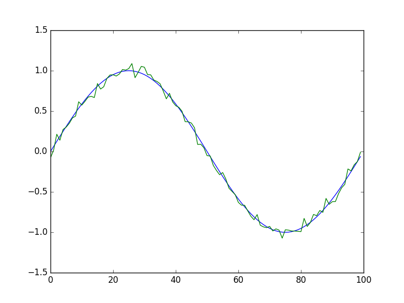
Complex mathematical expressions can be therefore specified very compactly using this property. For instance, in order to plot a sinewave with small additive normally-distributed noise, we can write:
import numpy as np
import matplotlib.pyplot as plt

# The x values
x = np.arange(100)

# The y values, uncorrupted
y = np.sin(2 * np.pi * np.arange(100) / 100.0)
plt.plot(x, y)

# The y values, now corrupted by Gaussian noise
y += np.random.normal(0, 0.05, size=100)
plt.plot(x, y)

plt.savefig("sin.png")
The result is:
Note
For the complete list of the available mathematical functions, see:
Linear Algebra
Numpy provides a number of linear algebraic functions, including dot products, matrix-vector multiplication, and matrix-matrix multiplication:
import numpy as np

# dot (scalar) product between vectors
x = np.array([0, 0, 1, 1])
print np.dot(x, x)

z = np.array([1, 1, 0, 0])
print np.dot(z, z)

print np.dot(x, z)

# Matrix-vector product
a = 2 * np.diag(np.ones(4))
print(np.dot(a, x))
print(np.dot(a, z))

# Matrix-matrix product
b = np.ones((4, 4)) - a
print(np.dot(a, b))
The result is:
# np.dot(x, x)
2

# np.dot(z, z)
2

# np.dot(x, z)
0

# np.dot(a, x)
[ 0.  0.  2.  2.]

# np.dot(a, z)
[ 2.  2.  0.  0.]

# np.dot(a, b)
[[-2.  2.  2.  2.]
 [ 2. -2.  2.  2.]
 [ 2.  2. -2.  2.]
 [ 2.  2.  2. -2.]]
Numpy also provides routines for dealing with eigenvalues/eigenvects, singular value decompositions, and other decompositions.
Let’s compute the (trivial) eigenvalues/eigenvectors of the 4x4 identity matrix:
>>> import numpy.linalg as la
>>> eigenvalues, eigenvectors = la.eig(np.ones((4, 4)))
>>> eigenvalues
array([ 0.,  4.,  0.,  0.])
>>> eigenvectors
array([[ -8.66025404e-01,   5.00000000e-01,  -2.77555756e-17,
         -2.77555756e-17],
       [  2.88675135e-01,   5.00000000e-01,  -5.77350269e-01,
         -5.77350269e-01],
       [  2.88675135e-01,   5.00000000e-01,   7.88675135e-01,
         -2.11324865e-01],
       [  2.88675135e-01,   5.00000000e-01,  -2.11324865e-01,
          7.88675135e-01]])
Note
The reference manual of the numpy.linalg module is here: